INDEX MATCH Function in Excel
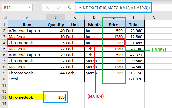
While the VLOOKUP function is widely used, it is known to be resource intensive and slow due to its inherent tendency to scan data columns from left to right, while performing a Lookup. In comparison, the hybrid INDEX MATCH Function is faster and more efficient due to its ability to go to the exact location of information, using a combination of INDEX and MATCH Functions. This GPS like accuracy is achieved by using INDEX function to identify ‘Data Array’ (where info to Lookup is located) and MATCH Function to pinpoint the location of Item (for which info is required).
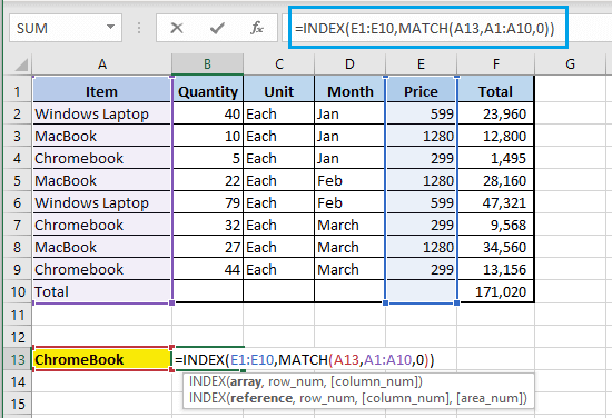
As you can see in above image, the INDEX Function identifies the location of Price Column and the Match Function pinpoints the Location of Item (Chromebook). So, let us go ahead and take a look at the steps to use INDEX and MATCH Functions in combination to perform a faster lookup.
1. How to Use INDEX MATCH Function in Excel
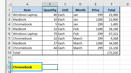
To illustrate the use of INDEX and MATCH Functions in combination, let us try to find the Price of MacBook from a Sales Data listing different types of computers sold along with their selling prices.
Type the Name of the item (MacBook) for which price is required in Cell A13.
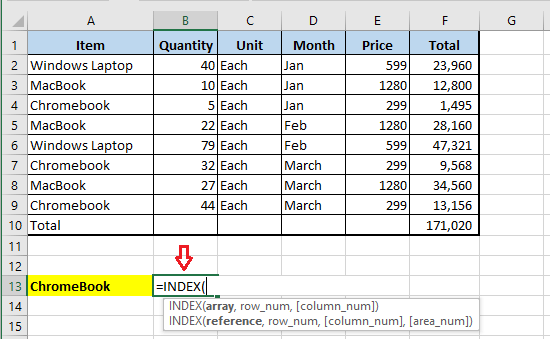
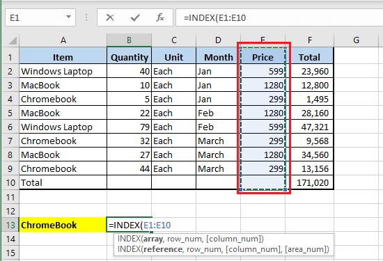
Next, place the curser in Cell B13 and start typing =INDEX – This will bring up the Syntax of Index Function.
Select E1:E10 as the INDEX Array – This is where the Price of items is located.
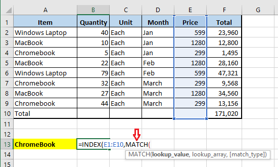
Now, instead of pointing to Row Number, type =Match – As we are going to use the Match Function to point to the location of Item Name (Chromebook) in our Data.
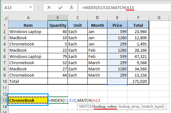
Note: Manually pointing to the Location of Item Name (Row, Col) is not easy in large data. Hence, the MATCH Function is being used to point to the exact location of Item Name. 5. Select, Cell A13 as the lookup_value – This is the item for which Price is required.
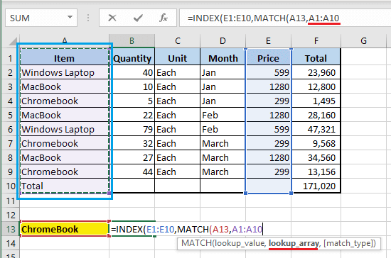
Select A1:A10 as the lookup_array – This is the range where item Names are located.
The next step is to state the Match Type – Select 0 – Exact Match.
Finally, close the Brackets and hit the Enter Key on the Keyboard of your computer.
Once you press the Enter Key, the INDEX MATCH Function will perform a Matrix search (Horizontally & Vertically) to bring the Price of Chromebook in Cell B13.
As you can see from above image, INDEX MATCH Function has scanned 2 data columns to find the Price of Chromebooks. In comparison, the VLOOK Function would have scanned 5 data columns to accomplish the same task.
How to Create Pivot Table in Excel How to Create Two Pivot Tables in Single Worksheet How to Use SUMIF Function in Excel