EXCEL SUMIFS Function
As you must be already aware, the SUMIF Function in Excel can be used to find the Sum, Count or the Total of items meeting a particular criteria or condition. Similarly, the SUMIFS Function in Excel can be employed to find the Sum or Total of items meeting not One but multiple criteria or conditions. For example, if there is sales data for different types of Gadgets sold at two different store locations, the SUMIFS Function can be used to count only iPads sold at the first store location. In above case, the SUMIFS Function counts only if the the Gadget type is iPad (First Criteria) and it is sold at the First Store (Second Criteria).
1. Syntax of Excel SUMIFS Function
The Syntax of SUMIFS Function is as provided below. =SUMIFS(sum_range, criteria_range1, criteria1, [criteria_range2, criteria2],…) Sum_range: The Range of Cells that you want to Sum. Criteria_range1: The range where the item meeting the first Criteria is located. Criteria1: The first condition or criteria, SUMIFS will be executed when these criteria is true. Criteria_range2: The range where the second item meeting the second Criteria is located. Criteria2: The second condition or criteria, SUMIFS will be executed when these criteria is true. As you can see from above, the Syntax of SUMIFS function allows you to specify multiple criteria and multiple ranges in which each of these criteria is located.
2. How to Use SUMIFS Function in Excel
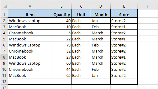
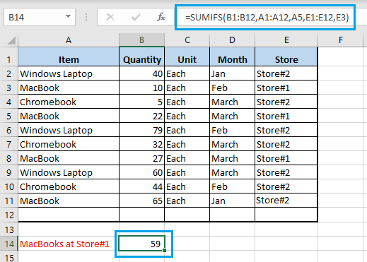
Take a look at the following table providing Sales Data for Windows Computers, ChromeBooks and MacBooks sold at two different store locations (Store#1 and Store#2).
The task is to find the total number of MacBooks sold at Store#1 using the SUMIFS Function in Excel.
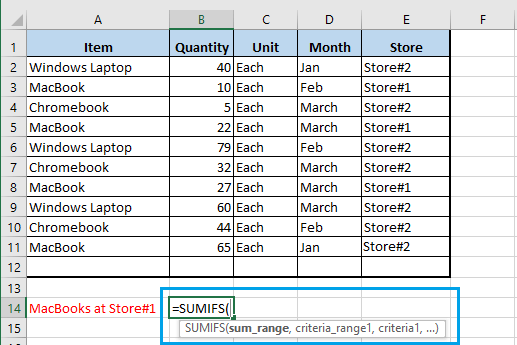
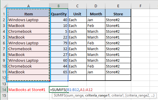
- Place the cursor in Cell B14 > start typing =SUMIFS and Microsoft Excel will automatically provide you with the Syntax to follow (=SUMIFS(sum_range, criteria_range1, criteria1, criteria_range2, criteria2,…).
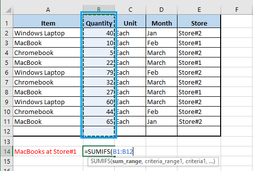
Note: Cell B14 is where you want to print the result. 2. Going by the Syntax, select Cells B1:B12 as the sum_range. This is where the items that you want to sum are located (number of items sold).
Next, select Cells A1:A12 as the criteria_range1 – this is where the first criteria (MacBook) is located.
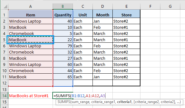
Select the First Criteria by clicking on Cell A5 containing the term ‘MacBook’.
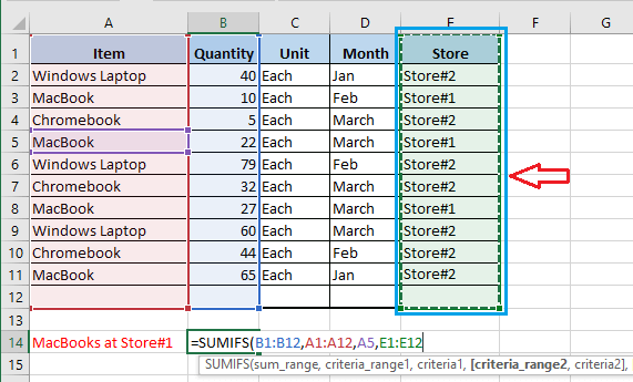
Select Cells E1:E12 as criteria_range2 – this is where the second criteria (Store#1) is located.
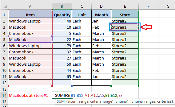
Now, select the Second Criteria by clicking on Cell E3 containing the term ‘Store#1’.
Finally, close the bracket and hit the enter key.
The SUMIFS formula will instantly display the number of MacBooks sold by Store#1 in cell B14.
How to Use COUNTIF Function in Excel How to Create Pivot Table in Excel How to Replace Zeros With Blank, Dash or Text in Excel