Create Waterfall Chart in Excel
Waterfall charts can be effectively used to illustrate the performance of an activity over a period of time, such as cash flows, operating costs, growth in customers, growth in population or the performance of an investment. In a typical Waterfall chart, the First and the Last columns represent the Total Start and Total End Values, while the intermediate floating columns represent the positive or negative contributions over a period of time. Waterfall charts were popularized by consulting firm McKinsey & Company which used them during their presentations to the clients.
Steps to Create Waterfall Chart in Excel
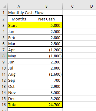
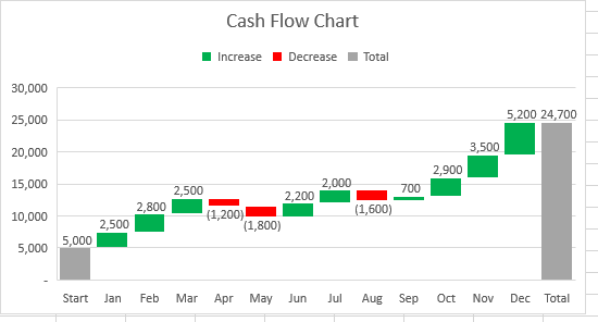
To explain the creation of Waterfall Charts in Excel, let us consider the hypothetical case of a business with an initial Cash of $5,000 at the beginning of the year and net monthly cash flows values for the next 12 months.
Just like in any business, the Net Monthly Cash Flows include both positive and negative numbers, depending on the difference between income and expenses in a given month. The first step in creating Waterfall Chart is to make sure that the given data has an Initial and an Ending value. In our case, the Ending Value ($24,700) is the sum total of Initial and Monthly cash values. Once you are satisfied with the data arrangement, you can follow the steps below to create Waterfall Chart in Excel.
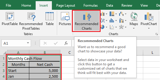
Select the Data that you want to create the Waterfall Chart from. 2. Next, click on the Insert tab and then click on Recommended Charts.
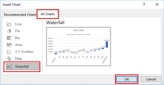
On Insert Chart screen, click on All Charts > Waterfall Chart option in the side menu and click on the OK button.
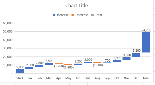
4. Once you click on OK, Microsoft Excel will automatically create a Waterfall Chart based on your data and the Chart will appear in the middle of your worksheet.
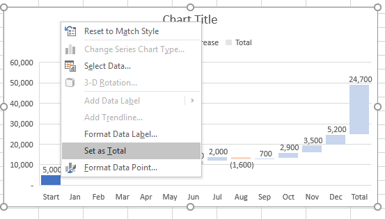
You can move the Waterfall Chart by dragging it and also change its size as required. 5. Now, to create Waterfall effect, you will have to set both Initial and End Data Points as Total Values. To do this, select the Initial value only (by double clicking on it), right-click on the Initial Value and click on Set as Total option.
Similarly, select the End Value, right-click on the End Value and click on Set as Total option in the menu that appears. 6. Once the Initial and End Values are fixed, you can Format the Waterfall Chart. In our case, we changed the colour of positive values to Green and Negative values to Red.
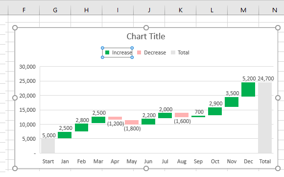
Tip: You can select all Negative or Positive Data points in the Chart by double-clicking on “Increase” and “Decrease” in the Legend (See image below).
After selecting data points, you will be able to change their Colour and Format them as required. As mentioned above, only Excel 2016 and later versions have to the ability to automatically create Waterfall Charts from a given data.
How to Create Pivot Tables in Excel How to use INDEX MATCH Function in Excel