Create Gantt Chart Using Excel
In simple terms, Gantt chart can be defined as a visual representation of activities or tasks scheduled over a period of time. In a typical Gantt Chart, the Horizontal axis (X-Axis) represents the time to complete the project, while the Vertical axis (Y-Axis) represents the activities or tasks required to complete the project. Depending on reporting requirements, the time span on the X-Axis is broken down into Days, Weeks or Months. Microsoft Excel does not offer a ready to use option or a template for Creating Gantt Charts. However, it is easy to Create Gantt Chart in Excel by modifying a Stacked bar Chart.
Steps to Create Gantt Chart in Excel
Follow the steps below to first insert a blank Stacked Bar Chart, add the required data to this chart and modify the resulting bar chart into a Gantt Chart Format.
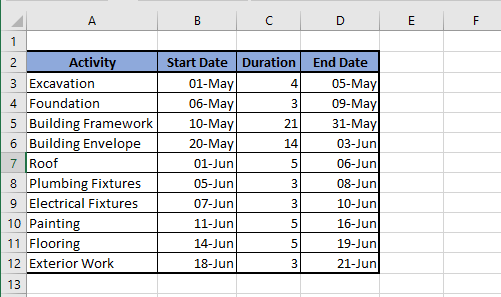
- The First step is to get your Data organized in an Excel worksheet.
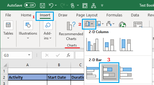
As you can see in above image, list of Activities, Start Dates and the Number of days required to complete individual activities have been listed in separate columns. 2. Now, click on the Insert tab, click on the Bar Chart icon (2) in ‘Charts’ section and select Stacked bar (3) option in the drop-down menu. This will insert a blank Stacked Bar Chart in your worksheet.
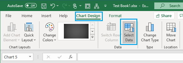
- Next, click on Chart Design tab and click on Select Data option located in the ‘Data’ section.
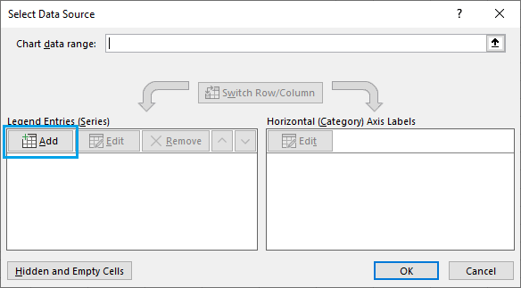
Note: If you do not see Chart Design tab, click on the empty Stacked bar chart in your worksheet. 4. In Select Data Source dialogue box that appears, click on the Add option.
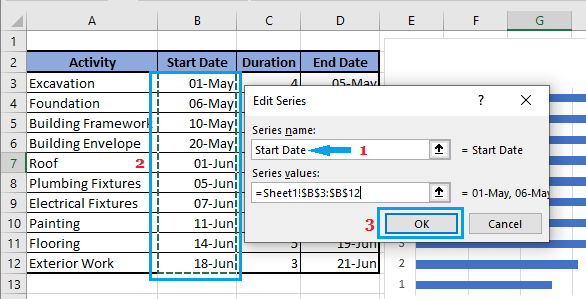
In Edit Series dialogue box, type Start Date (1) as Series Name, select Data range containing the Start Dates (2) as Series values and click on OK.
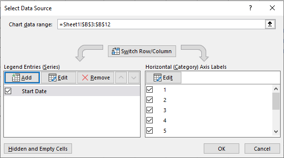
Click again on the Add option in select Data Source dialogue box.
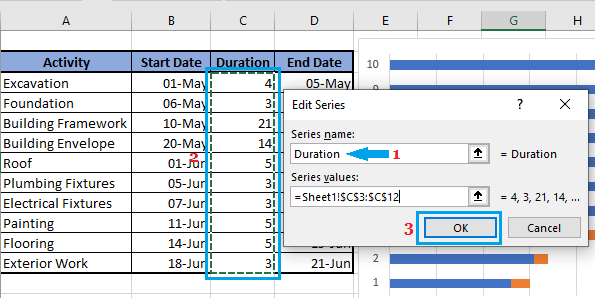
This time, type Duration (1) as the Series Name, select the data range containing Durations (2) and click on the OK button.
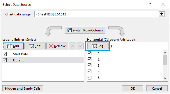
In ‘Select Data Source’ dialogue box, click on the Edit option located in the right-pane (Axis Labels).
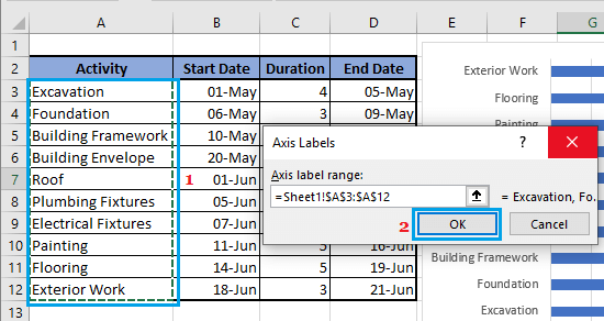
In Axis Label dialogue box, select the Data range containing the Activity Names (1) and click on OK.
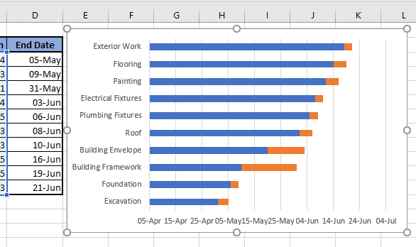
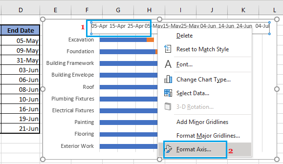
Click on OK to close the ‘Select Data Source’ dialogue box and you will end up with Stacked Bar Chart with activities in the reverse order.
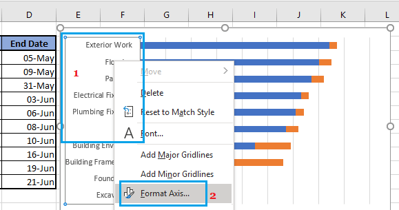
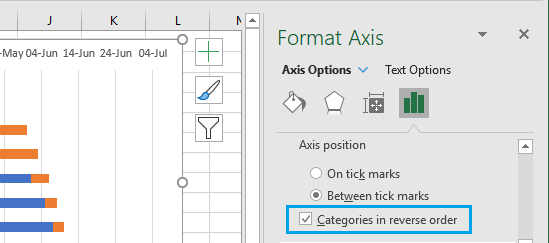
To correct the order, right-click on the Vertical Axis and select Format Axis option in the drop-down menu.
In Format Axis box that appears, scroll down to ‘Axis Position’ section and select Categories in reverse order option.
Now, right-click on the Horizontal Axis and select Format Axis option in the drop-down.
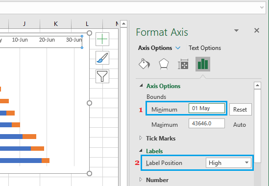
In Format Axis box, enter the Minimum Value as 01 May (Start Date of Project). After this, scroll down to the ‘Labels’ section and select High as the Label Position.
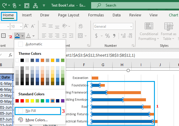
Finally, select the Blue bars in the Chart and remove the Colour Fill and Border (if present).
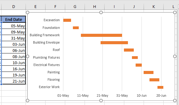
Your Gantt Chart is now ready.
You can change the Title and Format the Gantt Chart as required for your presentation or sending it for review.
How to Create Waterfall Chart in Excel How to Use VLOOKUP Function in Excel